library(devtools)
devtools::install_github("vanleeuwen-hans/concertData")
library(concertData)Multiple Setlist Alignment
Tour set-list alignment
Now we can dig a bit deeper, and see which songs are actually played in the set-lists of the shows within a tour. I have spent quite some time in experimenting with various biological sequence algorithms applied to this concert tour set-list alignment topic. For example, the CLUSTALW(Thompson, Gibson, and Higgins 2002) algorithms for multiple sequence alignment. The main challenge was to convert the non-biological sequence of a set-list to a biological sequence which is required for such algorithms. Eventually, I describe two approaches in this report:
custom R alignment code based on the Needleman-Wunsch(Murata 1990) algorithm
hybrid R-bash-R process with the MAFFT(Katoh 2002) algorithm
In the plots below you can very well see the conserved blocks of the show, as well as the moments when there is more variability in the song they play each night.
I also created an interactive Shiny app for this where you can select the tour of interest. See more info on the page Interactive Visualizations.
Load custom concertData package
First we load my custom concertData package where I organized all the functions to analyze the U2 concert data. This R package is available on my GitHub page at: https://github.com/vanleeuwen-hans/concertData.
Load the u2data
# read the u2 concertData
u2data <- read_concertData_csv('u2data/u2data_all_shows_clean_final.csv')
Set-list alignment with NW approach
The alignment plots below shows a first attempt of aligning setlists for each tour. It takes the 30 most representative shows for a tour, and then uses an alignment method to display the variation (or not) of songs played during the shows. The code handles insertions and deletions in the set-list sequences, similar to how DNA sequence alignment algorithms handle gaps. It uses dynamic programming to implement a variant of the Needleman-Wunsch(Murata 1990) algorithm.
# Filter for specific tour
tour_data <- u2data[u2data$tour == "U2 Vertigo Tour", ]
# Remove snippets
no_snippets_data <- concertData_remove_snippets(tour_data)
# Remove shows with no setlist
filtered_data <- concertData_remove_showsNoSetlist(no_snippets_data)

# Process the songs to create the mapping of codes
codes_tour_songs <- codify_tour_song_titles(filtered_data)

# create alignments using a customly written multiple setlist aligment code
# following the pairwise alignment approach of the Needleman-Wunsch algorithm
aligned_setlists <- create_setlist_alignment(filtered_data, max_shows = 30)

# create alignment data frame for downstream vizualisation
alignment_data <- format_alignment_data(aligned_setlists, codes_tour_songs, filtered_data)

# get number of shows in the alignment
num_setlists <- length(unique(alignment_data$showID))

# Mapping the sequence characters to the tour_song_codes
song_code_lookup <- codes_tour_songs[, c("hex_char", "four_letter_code", "song_title")]

# create vizualisation data object
viz_data <- create_setlist_viz_data(alignment_data, song_code_lookup, filtered_data)

# Create legend for acronyms/short titles
legend_data <- viz_data[!viz_data$is_gap, c("song_title", "four_letter_code")]
legend_data <- unique(legend_data)
legend_data <- legend_data[order(legend_data$song_title), ]
legend_text <- paste(legend_data$four_letter_code, "=", legend_data$song_title, collapse = ", ")

# Create custom color scale that uses distinct colors for songs and white for gaps
n_songs <- length(unique(viz_data$song_title[!viz_data$is_gap]))
song_colors <- create_distinct_palette(n_songs)
names(song_colors) <- unique(viz_data$song_title[!viz_data$is_gap])
song_colors <- c(song_colors, GAP = "white")

# Get the tour name from filtered_data
# Get a single showID from alignment_data
sample_showID <- alignment_data$showID[1]
# Lookup the tour_name in filtered_data
tour_name <- unique(filtered_data$tour[filtered_data$showID == sample_showID])

# plot the multiple sequence alignment of the tour setlists
# load library
library(ggplot2)
library(gridExtra)
library(stringr)

# Create a new column combining city and date
viz_data$city_date <- paste(viz_data$city, "-", as.character(viz_data$date))

# Create a unique identifier for each show
viz_data$show_id <- seq_len(nrow(viz_data))

# Convert city_date to a factor based on the original order in viz_data
viz_data$city_date <- factor(viz_data$city_date, levels = unique(viz_data$city_date[viz_data$show_id]))

# Create main plot
main_plot <- ggplot(viz_data, aes(x = position, y = city_date)) +
  geom_tile(aes(fill = song_title), color = "grey90", linewidth = 0.5) +
  geom_text(aes(label = ifelse(is_gap, "", four_letter_code)),
            size = 1.5,
            color = "white") +
  scale_fill_manual(values = song_colors) +
  theme_minimal() +
  theme(axis.text.x = element_text(angle = 90, hjust = 1, size = 7),
        axis.text.y = element_text(size = 8),
        plot.title = element_text(size = 12, hjust = 0.5),
        plot.subtitle = element_text(size = 10, hjust = 0.5),
        legend.position = "none",
        panel.grid = element_blank()) +
  labs(x = "Song Position", y = "City - Show Date",
       title = paste("Setlist Alignment for", tour_name),
       subtitle = paste("Showing", num_setlists, "most representative setlists. Empty white cells indicate inserted/skipped songs")
  )

# Create legend plot
legend_plot <- ggplot() +
  geom_text(aes(x = 0.5, y = 0.5, label = str_wrap(legend_text, width = 250)),
           size = 2, hjust = 0.5) +
  theme_void() +
  theme(plot.margin = margin(t = 10))

# Arrange plots together
grid.arrange(main_plot,
             legend_plot,
             ncol = 1,
             heights = c(4, 1))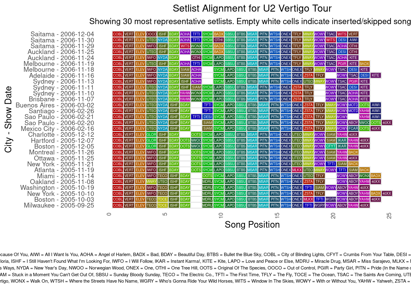
Multiple Setlist Alignment with MAFFT
I was not satisfied with the resulting alignments shown above, produced with the custom alignment code based on the Needleman-Wunsch algorithm. While exploring alternatives I discovered that the MAFFT(Katoh 2002) algorithm for multiple sequence alignment has an option ‘–text’ mode that can calculate and create multiple sequence alignments for non-biological sequences (see this page from the MAFFT authors). In the R package ips there is a mafft wrapper function, so I installed and tried it out. However, this R implementation of mafft does not allow for the --text mode. Hence, I implemented the solution using both R and the command line version of mafft on my Mac. I could also wrap the command line actions and execute it from R, but I did not spend time on that, mainly because it would still create a challenging dependency in my R-package.
When I first published this project report I had used the function ‘find_most_representative_setlists’ from my custom R package ‘concertData’. The function takes the setlists of all concerts in a tour, and was then supposed to identify the 30 setlists that represent best the overall variety seen in all the concerts of the tour. What it did was:
It used the Levenshtein distance to calculate similarities between setlists.
It computed a distance matrix for all pairs of setlists.
It calculated the average distance for each setlist to all others.
It selects the setlists with the lowest average distances as the most representative.
While this approach did identify setlists that are, on average, most similar to all other setlists, it did not fully achieve the stated goal for the following reasons:
Rare Changes: The method prioritizes setlists that are most similar to others, which means it might not capture rare changes or unique variations effectively. Rare changes would likely increase a setlist’s average distance, making it less likely to be selected.
Variety Representation: By selecting setlists with the lowest average distances, you’re essentially choosing the most “typical” setlists rather than those that represent the full variety of the tour.
Outlier Sensitivity: This method might be sensitive to outliers or very unique setlists, potentially skewing the results.
To better achieve the goal of representing all variety, including rare changes, I decided to use a clustering approach, with the k-means algorithm to group similar setlists, then select representatives from each cluster. Like this it better captures the full variety of setlists, including rare changes, while still maintaining a representative sample of the tour. This was implemented in the new function ‘find_representative_setlists_kmeans’ in my custom R package ‘concertData’ (see page: Sharing > concertData R package).
# Filter for specific tour
tour_data <- u2data[u2data$tour == "U2 Vertigo Tour", ]
# Remove snippets
no_snippets_data <- concertData_remove_snippets(tour_data)
# Remove shows with no setlist
filtered_data <- concertData_remove_showsNoSetlist(no_snippets_data)

# Process the songs to create the mapping of codes
codes_tour_songs <- codify_tour_song_titles(filtered_data)

# Prepare all setlist sequences
all_setlist_sequences <- prepare_setlist_sequences(filtered_data, codes_tour_songs)

# Find the most representative setlists
#representative_setlists <- find_most_representative_setlists(all_setlist_sequences, n_representatives = 30)
representative_setlists <- find_representative_setlists_kmeans(all_setlist_sequences, n_representatives = 30)

# Create fasta-format sequences representing the set-lists of the representative shows
fasta_mafft_output <- create_setlist_fasta_mafft(representative_setlists)
writeLines(fasta_mafft_output, "mafft/u2_setlists.hex")
Now we have the FASTA-like file with hex values that we can use as input for the multiple sequence alignment algorithm MAFFT. See explanation for this text mode version (non-biological sequences alignment) at: https://mafft.cbrc.jp/alignment/software/textcomparison.html
Following the flow explained there, we convert the HEX file to ASCII code using the hex2mafftext command:
hex2maffttext u2_setlists.hex > u2_setlists.ASCIIThe resulting file looks like:
head u2_setlists.ASCII
>showID1392
,Q9R87,HL9M8CKVJMNf8I^_
>showID1408
,Q9NM7,HL9M8CKVJROf8I^_
>showID1328
,Q9E87,HL9M8CKVJG7f8I^_
>showID1320
,Q9887,HL9M8CKVJGYf8I^_
>showID1325
,Q9E87,HL9M8CKVJROf8I+^_
Then we run the actual multiple sequence alignment with the command:
mafft --text --clustalout u2_setlists.ASCII > u2_setlists_mafft_alignment.ASCIIThe output of the run:
nthread = 0
nthreadpair = 0
nthreadtb = 0
ppenalty_ex = 0
stacksize: 8192 kb
nalphabets = 256
Gap Penalty = -1.53, +0.00, +0.00


Making a distance matrix ..
    1 / 30
done.

Constructing a UPGMA tree (efffree=0) ...
   20 / 30
done.

Progressive alignment 1/2...
STEP    20 / 29  d
Reallocating..done. *alloclen = 1048
STEP    29 / 29  h
done.

Making a distance matrix from msa..
    0 / 30
done.

Constructing a UPGMA tree (efffree=1) ...
   20 / 30
done.

Progressive alignment 2/2...
STEP    28 / 29  d
Reallocating..done. *alloclen = 1048
STEP    29 / 29  h
done.

disttbfast (text) Version 7.526
alg=A, model=Extended, 1.53, -0.00, -0.00, noshift, amax=0.0
0 thread(s)


Strategy:
 NW-NS-2 (Fast but rough)
 Progressive method (guide trees were built 2 times.)

If unsure which option to use, try 'mafft --auto input > output'.
For more information, see 'mafft --help', 'mafft --man' and the mafft page.

The default gap scoring scheme has been changed in version 7.110 (2013 Oct).
It tends to insert more gaps into gap-rich regions than previous versions.
To disable this change, add the --leavegappyregion option
The output sequence alignment file looks like this:
more u2_setlists_mafft_alignment.ASCII
CLUSTAL format alignment by MAFFT NW-NS-2 (v7.526)


showID1392      -,Q9R-87,HL9M8CKVJMN-f8I^_-
showID1408      -,Q9N-M7,HL9M8CKVJRO-f8I^_-
showID1328      -,Q9E-87,HL9M8CKVJG7-f8I^_-
showID1320      -,Q98-87,HL9M8CKVJ-GYf8I^_-
showID1325      -,Q9E-87,HL9M8CKVJRO-f8I+^_
showID1299      -,Q9D-8,-HL9M8\KVJRO-Nf8^_-
showID1286      -,Q9R-88,HL9M8\KVJRO-N8^_--
showID1282      -,Q9R-8,-HL9M8\KVJRO-N8^_--
showID1339      -,Q9E--7,UL9M8CKVJMN-f7I^_-
showID1412      -,Q9D--7,UL9M8CKVJMN-f7I^_-
showID1327      -,Q9E-87,HL9M8CKVJ(--f8^_--
showID1271      QE899-,7,HL9M8CKVJRO-f8^_--
showID1267      QE899-,7,HL9M8CKVJRO-f8Q--
showID1269      QE899-,7,HL9M8CKVJRO-f8Q--
showID1270      QE899-,7,HL9M8CKVJRO-f8Q--
showID1393      -,Q9E-87,UL9M8CKVJMO-f8\+-
showID1321      -,Q98-87,HL9M8CKVJLGYf8I^_-
showID1331      -,Q9E887,HL9M8CKVJ\7-f8I^_-
showID1330      -,Q9E-87,HL9M8CKVJG7Bf8I^_-
showID1336      -,Q9N-M7,HL9M8CKVJ7Y-f8I^_-
showID1329      -,Q9-8@7,HL9M8CKVJ\Y-f8+--
showID1259      QE89,-77,HL9M8CKVJRO-f8Q--
showID1266      QE899-,7,HL9M8CKVJRO-f8BQ-
showID1289      QE899-,7,HL9M8CKVJRO-f8BQ-
showID1435      -,Q9E--9,DL9M8CKVJON-f8%:-
showID1281      -,Q9R-8,9HL9M8\KVJRO-N8^_--
showID1305      -,Q9R-8,9HL9M8\KVJRO-N8^_--
showID1436      -,Q9E-9,7%L9M8CKVJRO-f82:-
showID1322      -,Q988F7,HL9M8CKVJG7-f8^_--
showID1284      -,Q9D-8,-HL9M8\KVJRO-N87+-
                   *      **** ***
Now we can visualize this multiple set list alignment. We see that the alignment is of better quality than the NW- based method in the previous paragraph. It is still not perfect and perhaps tweaking the MAFFT algorithm parameters could further improve it. I developed a Shiny App where you can see the alignments for all major U2 tours, see the [Interactive Visualizations](interactive-visual-apps.qmd) page.
# libraries
library(dplyr)
library(stringr)

# Get a data frame from the mafft clustal output
alignment_data <- read_mafft_clustal_alignment("mafft/u2_setlists_mafft_alignment.ASCII")

# get number of shows in the alignment
num_setlists <- length(unique(alignment_data$showID))

# Mapping the sequence characters to the tour_song_codes
song_code_lookup <- codes_tour_songs[, c("hex_char", "four_letter_code", "song_title")]

# create vizualisation data object
viz_data <- create_setlist_viz_data(alignment_data, song_code_lookup, filtered_data)

# Create legend for acronyms/short titles
legend_data <- viz_data[!viz_data$is_gap, c("song_title", "four_letter_code")]
legend_data <- unique(legend_data)
legend_data <- legend_data[order(legend_data$song_title), ]
legend_text <- paste(legend_data$four_letter_code, "=", legend_data$song_title, collapse = ", ")

# Create custom color scale that uses distinct colors for songs and white for gaps
n_songs <- length(unique(viz_data$song_title[!viz_data$is_gap]))
song_colors <- create_distinct_palette(n_songs)
names(song_colors) <- unique(viz_data$song_title[!viz_data$is_gap])
song_colors <- c(song_colors, GAP = "white")

# Get the tour name from filtered_data
# Get a single showID from alignment_data
sample_showID <- alignment_data$showID[1]
# Lookup the tour_name in filtered_data
tour_name <- unique(filtered_data$tour[filtered_data$showID == sample_showID])

# plot the multiple sequence alignment of the tour setlists
# load library
library(ggplot2)
library(gridExtra)

# Create a new column combining city and date
viz_data$city_date <- paste(viz_data$city, "-", as.character(viz_data$date))

# Create a unique identifier for each show
viz_data$show_id <- seq_len(nrow(viz_data))

# Convert city_date to a factor based on the original order in viz_data
viz_data$city_date <- factor(viz_data$city_date, levels = unique(viz_data$city_date[viz_data$show_id]))

# Create main plot
main_plot <- ggplot(viz_data, aes(x = position, y = city_date)) +
  geom_tile(aes(fill = song_title), color = "grey90", linewidth = 0.5) +
  geom_text(aes(label = ifelse(is_gap, "", four_letter_code)),
            size = 1.5,
            color = "white") +
  scale_fill_manual(values = song_colors) +
  theme_minimal() +
  theme(axis.text.x = element_text(angle = 90, hjust = 1, size = 7),
        axis.text.y = element_text(size = 8),
        plot.title = element_text(size = 12, hjust = 0.5),
        plot.subtitle = element_text(size = 10, hjust = 0.5),
        legend.position = "none",
        panel.grid = element_blank()) +
  labs(x = "Song Position", y = "City - Show Date",
       title = paste("Setlist Alignment for", tour_name),
       subtitle = paste("Showing", num_setlists, "most representative setlists. Empty white cells indicate inserted/skipped songs")
  )

# Create legend plot
legend_plot <- ggplot() +
  geom_text(aes(x = 0.5, y = 0.5, label = str_wrap(legend_text, width = 250)),
           size = 2, hjust = 0.5) +
  theme_void() +
  theme(plot.margin = margin(t = 10))

# Arrange plots together
grid.arrange(main_plot,
             legend_plot,
             ncol = 1,
             heights = c(4, 1))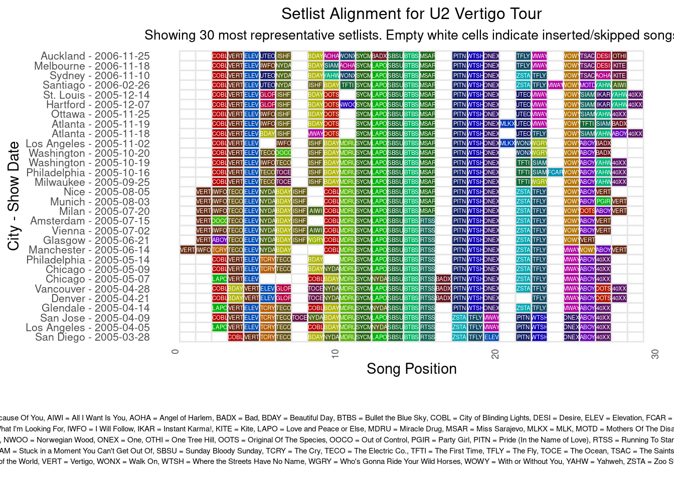
Distance tree of aligned setlists
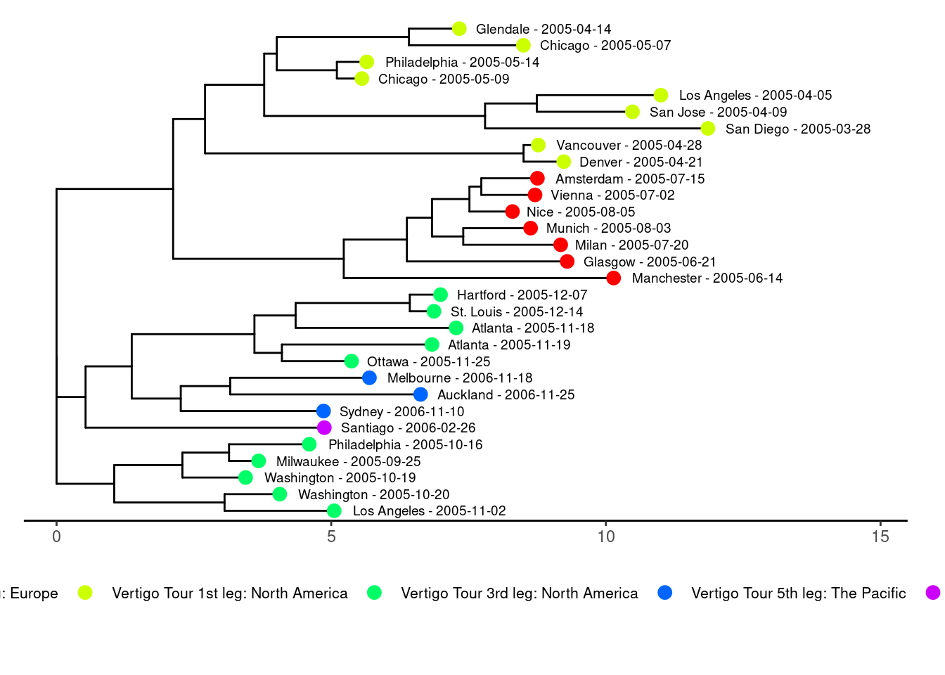
Another way to display the relatedness of setlists is to use a distance tree, often used for biological sequences, producing so called phylogenetic trees. The ggtree(Xu et al. 2022) and ape(Paradis and Schliep 2018) packages were used for the plots. In the plot with the tree tips colored by tour leg, you can clearly see that setlists from the same leg tend to be more similar.
library(dplyr)
library(seqinr)
library(ape)
library(ggplot2)
library(ggtree)

# Get a data frame from the mafft clustal output
alignment_data <- read_mafft_clustal_alignment("mafft/u2_setlists_mafft_alignment.ASCII")
# Convert data frame to list which is needed for downstream distance tree analysis
sequences <- setNames(as.list(alignment_data$sequence), paste0("showID", alignment_data$showID))

# Calculate distance matrix
dist_matrix <- calculate_distance_matrix(sequences)
# Convert to dist object
setlist_dist <- as.dist(dist_matrix)
# Construct the tree
setlist_tree <- nj(setlist_dist)

# Collect show info
show_info <- unique(filtered_data[, c("showID", "city", "date", "country", "leg")])
show_info$city_date <- paste(show_info$city, format(show_info$date, "%Y-%m-%d"), sep = " - ")

# create tree labels in the format 'City YYYY-MM-DD'
new_labels <- create_city_date_tree_labels(filtered_data, setlist_tree, show_info)
# Modify tree labels
setlist_tree$tip.label <- new_labels

# create standard tree plot
tree_plot <- create_ggtree_plot(setlist_tree)
# Display the plot
print(tree_plot)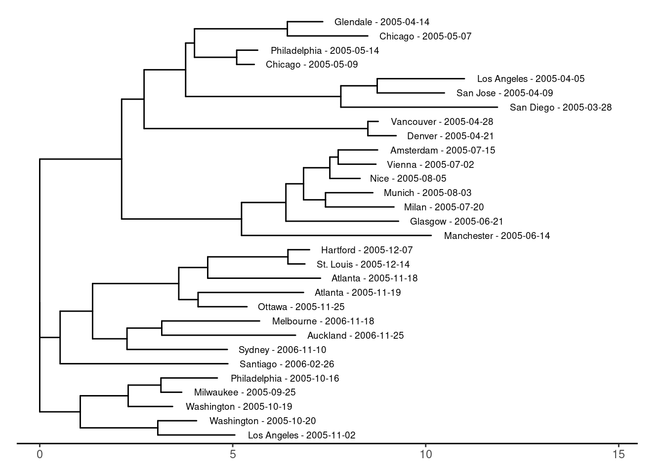
# Create the tree plot with colors based on country
plot_country <- create_ggtree_plot_colored(setlist_tree, show_info, color_by = "country")
print(plot_country)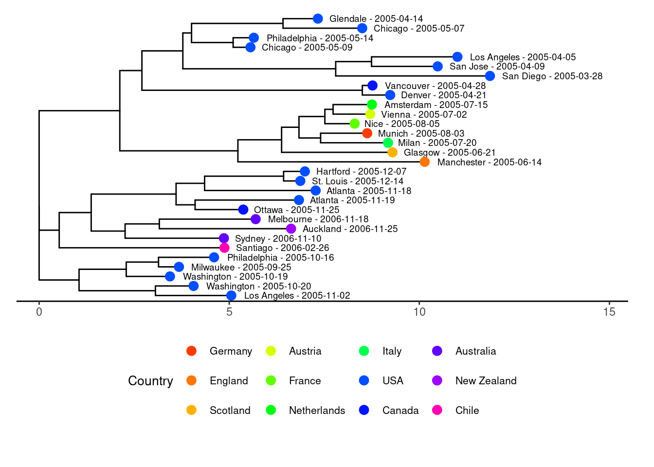
# Create the tree plot with colors based on leg
plot_leg <- create_ggtree_plot_colored(setlist_tree, show_info, color_by = "leg")
print(plot_leg)